6. Phase transitions
6.1. Nucleation and growth
In the first half of the 18th century, the Swedish scientist Anders Celsius developed a temperature scale that is now named after him. Orginally he defined the boiling point of water at a pressure of 1 atm (\(\approx 10^5 \;\mathrm{Pa}\)) to be 0 degrees, and the freezing point to be 100 degrees. Shortly after, the scale was reversed by the French scientist Christin, and independently by the Swedish botanist Carl Linnaeus. The Celsius and Kelvin scale are essentially identical, in the sense that a temperature difference of \(1\;^\mathrm{o}\mathrm{C}\) is equal to a difference of \(1 \;\mathrm{K}\), except that the absolute values are shifted, \(0\;^\mathrm{o}\mathrm{C}=273.15 \;\mathrm{K}\).
During phase transitions such as freezing and boiling the molecules of a substance radically change their configuration or density. These transitions can be induced by a change in temperature or pressure, or by external fields. During the process of freezing, the molecules in a liquid phase lose their ability to diffuse and get trapped in an ordered, crystalline lattice. This usually happens by a process called “nucleation and growth” where a small nucleus of frozen molecules grows larger and larger over time, after overcoming a “nucleation barrier”. To overcome this energy barrier, nuclei first need to grow large enough by thermal fluctuations before they can grow spontaneously (i.e. before growth leads to a lowering of the free energy). If the temperature of the environment is not too low, the nucleation barrier may be sufficiently high to prevent multiple nuclei overcoming the nucleation barrier. In that case, the new phase will grow from a single nucleus and may have a high degree of symmetry. On the other hand, if multiple nuclei start growing at the same time, the resulting phase may consist of many crystalline domains, separated by fault lines and defects. For some applications, this may be highly desirable, while for others it is not (see exercise). Fig. 6.1 shows a liquid crystal, frozen into different crystalline domains.

Fig. 6.1 Crystal domains of a liquid crystal. In each domain, the crystal structure has a different orientation.
A phase transition can also happen by another type of process, where the transition happens spontaneously, everywhere, and almost instantaneously. This process has the fancy name of “spinodal decomposition”, and happens after one disturbs a supercooled phase. This phenomenon is responsible for freezing rain. Under special weather conditions, rain drops can be cooled below the freezing temperature of water on their way to the earth’s surface, and hit the ground before they have the time to freeze via nucleation. The shockwave of the impact is sufficient to start the phase transition at every point at the same time, making the droplet freeze in an instant. This phenomenon may be beautiful to behold, but can, understandably, also be a major disturbance for traffic and infrastructure. In northern places where this phenomenon is more common, it is feared by trees and electricity lines.
In discussions about phase transitions, water seems a natural example, because of its abundance and relevance for life, and our experience with its behavior, but it has many exceptional properties that other substances do not have, and some of them are still not understood. We will skip that discussion for now.
Recipes usually recommend adding salt to boiling water before adding pasta, to make the pasta less sticky. When one adds salt to boiling water, it usually produces a short burst of bubbles. Why would this happen?
Why is it important to “temper” chocolate (i.e. to cool it very slowly below its freezing point)? Name at least two reasons.
What preparations are important if one wants to make a dessert with supercooled water? Name at least three important measures.
Some types of frogs can freeze for an entire winter. About 70% of the water in their body freezes completely. When the nights turn colder, the frogs produce a special type of protein that regulates the formation of ice crystals in their body, in places where water is allowed to freeze. To prevent desiccation via osmosis, their body also produces higher levels of glucose. Eventually their heartbeat and breathing come to a complete standstill, and they are basically dead, until spring returns.
Why is frost so harmful for other creatures? And why is frozen food so soft? (this may be one of the reasons why one should not eat kale before the first night of frost, as old wisdom says.)
The Gibbs free energy of a solid nucleus is approximated by
\[ G = 4\pi R^2 \gamma - \frac{4\pi R^3}{3} \Delta G \]with \(R\) the radius of the nucleus, \(\gamma\) the surface tension between the nucleus and the continuum phase, and \(\Delta G\) the (free) energy difference between the solid and liquid phase. Calculate how large a nucleus needs to grow before it can grow spontaneously, in terms of \(\gamma\) and \(\Delta G\). Call the corresponding critical radius \(R_\mathrm{crit}\).
6.2. Van der Waals fluids
This question will not be about “Van der Waals forces”, a type of interaction that acts between every type of atom and molecule, and tends to be attractive. These forces make molecules attract each other, and make nature at its smallest scales rather ‘sticky’. The origin of these forces is electromagnetic. Electrons orbiting the nucleus of an atom create temporal dipole moments, and these moments can couple to that of other atoms. But let us not get into all the subtleties of these forces (and there are quite a few).
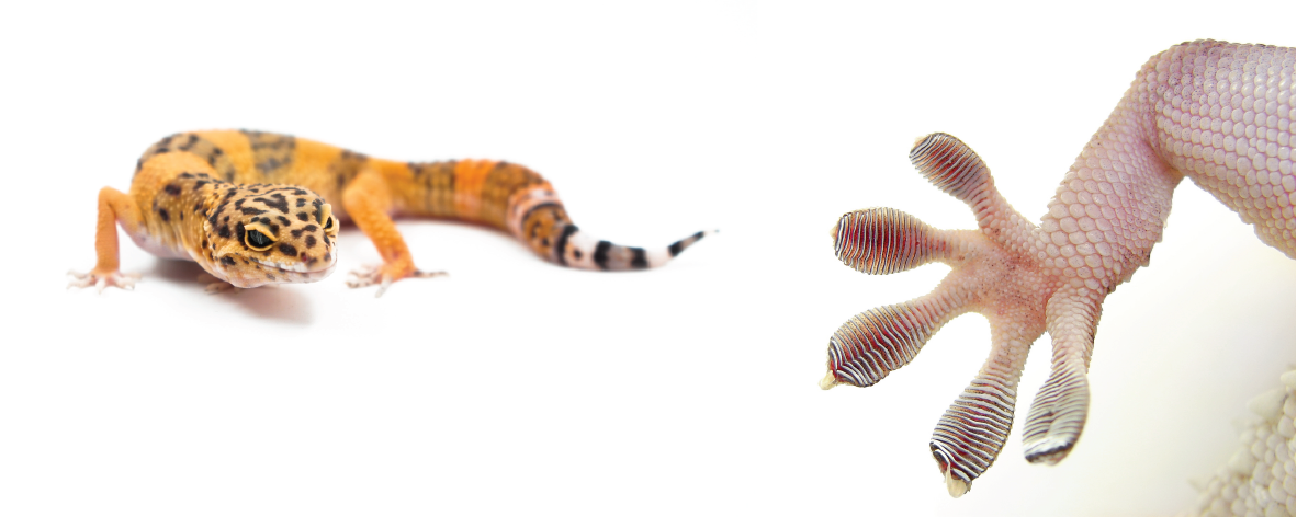
Fig. 6.2 A gecko can scale walls thanks to sticky Van der Waals forces. Their feet have a lot of grooves to increase their surface area. Research groups have tried to imitate their art to create ‘spider man suits’ for human beings. Unfortunately, the ratio between our body weight and surface area is not optimal for this ability. Images by Verdian Chua on Unsplash and Matt Reinbold on Flickr.
Johannes van der Waals tried to understand why fluids can decide to separate into two phases, a dense liquid phase, and a dilute gas phase. He constructed a model, based on the ideal gas, but with two extra modifications. One modification was to change the volume \(V\) by subtracting the volume occupied by the fluid (effectively giving the particles a ‘size’ such that they can collide with each other), and the other modification was to make the fluid cohesive (equivalent to adding attractive forces between the particles). His model predicted that such fluids can phase separate, if the temperature is sufficiently low, and that there is a ‘critical temperature’ and ‘critical density’ where the fluid is just about to separate. This exercise will guide you through his model. James Clerk Maxwell was so curious to learn about his work and his thesis in particular, that he decided to learn Dutch.
Van der Waals modified the free energy of an ideal gas
to
The second term, containing the parameter \(a\), represents cohesion. One can see that this term lowers the free energy as the density gets larger. In the first term, the volume is adapted by a parameter \(bN\), where \(b\) represents the size of a particle.
The pressure can be calculated by the fundamental relation
\[ p = - \frac{\partial F}{\partial V}. \]Calculate the pressure of the ideal gas and of a Van der Waals fluid.
Plot the ideal gas pressure and that of a van der Waals fluid as a function of density \(\rho = \frac{N}{V}\), for two values of \(a\): \(a=0\) and \(a>0\). You can use graphic calculators, Wolfram Alpha, or any tool you like, or just the mental skills. You can set \(k_\mathrm{B}T\) to 1 if you prefer.
In the previous question, you may have noticed that the pressure may decrease with density, if \(a\) is sufficiently large. What does this mean? (Try to imagine what would happen if a small fluctuation in density would occur.)
If the pressure as a function of density has maxima and minima, it is a sign that the fluid may separate into two phases. One condition for phase coexistence is that the pressures of the two phases need to be the same (this comes down to Newton’s first law) Sketch o new plot \(p\) vs. \(\rho\) (with sufficiently large \(a\)) and indicate the interval of densities where you could expect a phase coexistence.
The other condition for phase coexistence is that the chemical potentials of the two phases need to be the same;
\[ \mu = \frac{\partial F}{\partial N}. \]Calculate the chemical potential of the ideal gas and of a Van der Waals fluid.
Plot the chemical potential of the ideal gas and that of a van der Waals fluid as a function of density, for two values of \(a\): \(a=0\) and \(a>0\). If you used a computational tool to generate the graph of \(p\) vs. \(\rho\), use the same value of \(a\) to calculate the chemical potential.
Is there an interval where you could expect a phase coexistence, if you look at the graph of the chemical potential vs. density?
There is a clever method to check whether a fluid will phase separate, and if so, what the two coexisting densities will be. Those two densities should have the same pressure and chemical potential.
First let us introduce the free energy density \(f\), defined as \(f\equiv \frac{F}{V}\). Show that
\[ f_\mathrm{VdW} = k_\mathrm{B}T\rho \left( \ln{\frac{\rho}{1-b\rho}} -1 \right) - a \rho^2. \]From the definition of \(f = \frac{F}{V}\), derive that
(6.1)¶\[ \mu = \frac{\partial f}{\partial \rho} \]and
(6.2)¶\[ p = \rho \frac{\partial f}{\partial \rho} - f. \]Hint: it may be useful to substitute \(F=Vf\), and to use the chain rule
\[ \frac{\partial}{\partial V} = \frac{\partial \rho}{\partial V}\frac{\partial}{\partial \rho} \]to derive the equations.
If you would plot \(f\) as a function of density, the graph may look something like Fig. 6.3, depending on the value of \(a\). Then, if you would put your ruler against the graph, to draw a straight line connecting two points with the same slope, by a straight line with the same slope, you would get the black line shown in Fig. 6.3. Using equations (6.1) and (6.2), argue that the two points, \(\rho_1\) and \(\rho_2\) have the same pressures and chemical potentials.
%config InlineBackend.figure_formats = ['svg']
import numpy as np
import matplotlib.pyplot as plt
from myst_nb import glue
from scipy.optimize import fsolve
# Global parameters
kbt = 1 # --> all energy (f, a, ...) in units of k_B T
linear_coefficient = 2.5 # add a term linear in rho to f_vdw for a nicer plot
# this linear term has no impact on the conditions for phase coexistence
# Colors
grey = '#eeeeee' # light grey fill
line = '#e96868' # red line
nucleatn_color = '#6a8ba4' # dark blue for nucleation&growth
spinodal_color = '#BBDEF0' # light blue for spinodal decomposition
def f_vdw(rho, a, b):
"""
Calculates the free energy density for a Van der Waals fluid.
"""
return kbt*rho*(np.log(rho/(1-b*rho)) - 1) - a*rho**2 + linear_coefficient*kbt*rho
def f_vdw_prime(rho, a, b):
"""
Calculates the derivative w.r.t. the density rho of the free energy
density of a VdW fluid.
"""
return kbt*np.log(rho/(1-b*rho)) + kbt*b*rho/(1-b*rho) - 2*a*rho + linear_coefficient*kbt
def conditions_for_coexistence(x, a, b):
"""
Function that should be zero when phases coexist. A vector with
one element mu1 - mu2, and one element p1 - p2.
"""
rho1 = x[0]
rho2 = x[1]
mu1 = f_vdw_prime(rho1, a, b)
mu2 = f_vdw_prime(rho2, a, b)
f1 = f_vdw(rho1, a, b)
f2 = f_vdw(rho2, a, b)
mu_deficit = mu1 - mu2
p_deficit = rho1*mu1 - f1 - rho2*mu2 + f2
return [mu_deficit, p_deficit]
def f_mix(rho_av, a, b):
"""
Free energy density for a mixture of gas (density rho1) and liquid (density
rho2). The gas and liquid densities (rho1 and rho2) are found numerically.
"""
rhosol = fsolve(conditions_for_coexistence, x0=[0.05, 0.7], args=(a,b))
rho1 = rhosol[0]
rho2 = rhosol[1]
return f_vdw(rho1, a, b) + (f_vdw(rho2, a, b) - f_vdw(rho1, a, b))/(rho2-rho1) * (rho_av - rho1)
## Prepare all the graphs that are to be plotted
# Define the range of densities to plot
rho = np.linspace(0.001, 0.95, 1000)
# Set the parameters a and b
a = 4
b = 1
# Find the densities at which the gas and liquid phases coexist by solving
# numerically. If you use different a and b you might need to change the
# guesses, x0.
rhosol = fsolve(conditions_for_coexistence, x0=[0.05, 0.8], args=(a,b))
## Make the plot
fig, ax = plt.subplots(figsize=(6,4))
# Put axes on the zeros
ax.spines['left'].set_position('zero')
ax.spines['right'].set_color('none')
ax.spines['bottom'].set_position('zero')
ax.spines['top'].set_color('none')
ax.xaxis.set_ticks_position('bottom')
ax.yaxis.set_ticks_position('left')
# Remove label at 0.0
ax.set_xticks([0.2, 0.4, 0.6, 0.8])
# Plot the graphs
ax.plot(rho, f_vdw(rho, a, b), color=line)
ax.plot(rho, f_mix(rho, a, b), 'k')
# Create markers rho1 and rho2
rho1_marker_y = np.linspace(0, f_vdw(rhosol[0], a, b), 10)
rho1_marker_x = np.ones(rho1_marker_y.shape)*rhosol[0]
ax.plot(rho1_marker_x, rho1_marker_y, 'k--')
rho2_marker_y = np.linspace(0, f_vdw(rhosol[1], a, b), 10)
rho2_marker_x = np.ones(rho2_marker_y.shape)*rhosol[1]
ax.plot(rho2_marker_x, rho2_marker_y, 'k--')
ax.text(rhosol[0], 0.01, r'$\rho_1$')
ax.text(rhosol[1], 0.01, r'$\rho_2$')
# Labels
ax.set_xlabel(r'density $\rho$'), ax.set_ylabel(r'free energy density $f$')
# Limits
ax.set_xlim([0, rho[-1]])
ax.set_ylim([-0.4, 0.05])
# Save graph to load in figure later (special Jupyter Book feature)
glue("free_energy_density", fig, display=False)

Fig. 6.3 The free energy density (blue curve), with a “common tangent construction” (black straight line), connecting two points with the same slope, by a straight line with the same slope.
The region in between these two points is ‘unstable’. If you would prepare a system with an intermediate density, it could separate into the two coexisting densities, found in the previous question. Fig. 6.4 shows that the free energy of a phase separated system is lower than that of a homogeneous system, if the average density of the phase-separated mixture is \(\rho_1<\rho_\mathrm{average}<\rho_2\) 1.
However, to separate completely, a homogeneous system may have to overcome an energy barrier to do so. This happens in the regime where \(f\) is convex (the second derivative is positive). In that regime, small fluctuations in the density have a higher free energy than the homogeneous phase (draw a straight line between two points on a convex curve to see how that works).
But when \(f\) is concave, any tiny fluctuation will lower the free energy, and the separation would occur spontaneously. This happens during “spinodal decomposition”, e.g. when you disturb a supercooled liquid.
Fig. 6.5 shows the regimes where these processes take place. Usually it is the temperature that induces a transition. By lowering the temperature, the parameter \(a/k_\mathrm{B}T\) increases, and the free energy curve changes. If you want to supercool a liquid, it is advisable to do it quickly, in a clean bottle, to prevent the nucleation process, and to cool it fast to a low temperature (\(<-18^\mathrm{o}\)C) to make sure that the water ends up in the highly unstable regime (blue shaded region in Fig. 6.5). Any tiny perturbation will then initiate the separation process.
At the bottom of this page, you can find an interactive plot for the free energy density where you can vary the parameter \(a\).
fig2, ax = plt.subplots(figsize=(6,4))
# Put axes on the zeros
ax.spines['left'].set_position('zero')
ax.spines['right'].set_color('none')
ax.spines['bottom'].set_position('zero')
ax.spines['top'].set_color('none')
ax.xaxis.set_ticks_position('bottom')
ax.yaxis.set_ticks_position('left')
# Remove label at 0.0
ax.set_xticks([0.2, 0.4, 0.6, 0.8])
# Grey area
ax.fill([rhosol[0], rhosol[0], rhosol[1], rhosol[1]],
[0, -0.4, -0.4, 0],
color=grey)
# Plot the graphs
ax.plot(rho, f_vdw(rho, a, b), color=line, label='homogeneous density')
ax.plot(rho, f_mix(rho, a, b), 'k', label='phase separated')
# Create markers for rho1 and rho2
ax.scatter(rhosol[0], 0, color='k', marker='|', zorder=10)
ax.scatter(rhosol[1], 0, color='k', marker='|', zorder=10)
ax.text(rhosol[0], 0.01, r'$\rho_1$', zorder=10)
ax.text(rhosol[1], 0.01, r'$\rho_2$', zorder=10)
# Create markers for rho_average
rhoavg = 0.3
rhoavg_marker_y = np.linspace(0, f_mix(rhoavg, a, b), 10)
rhoavg_marker_x = np.ones(rho1_marker_y.shape)*rhoavg
ax.plot(rhoavg_marker_x, rhoavg_marker_y, 'k--')
fmix_at_rhoavg = f_mix(rhoavg, a, b)
fvdw_at_rhoavg = f_vdw(rhoavg, a, b)
hline_x = np.linspace(0, rhoavg, 10)
mix_hline_y = np.ones(hline_x.shape)*fmix_at_rhoavg
vdw_hline_y = np.ones(hline_x.shape)*fvdw_at_rhoavg
ax.plot(hline_x, mix_hline_y, 'k--')
ax.plot(hline_x, vdw_hline_y, '--', color=line)
ax.text(rhoavg, 0.01, r'$\rho_\mathrm{average}$')
# Labels
ax.set_xlabel(r'density $\rho$'), ax.set_ylabel(r'free energy density $f$')
# Limits
ax.set_xlim([0, rho[-1]])
ax.set_ylim([-0.4, 0.05])
# Legend
ax.legend()
# Save graph to load in figure later (special Jupyter Book feature)
glue("free_energy_density_again", fig2, display=False)

Fig. 6.4 The free energy density of a homogeneous system (blue curve) plotted against the density, and of a phase separated system (points on the black line, in between \(\rho_1\) and \(\rho_2\)), plotted against its mean density \(\rho_\mathrm{average}\).
def f_vdw_doubleprime(rho, a, b):
"""
Calculates the second derivative of the free energy density for a
Van der Waals fluid.
"""
return kbt/(rho*(1-b*rho)) + kbt*b/(1-b*rho)**2 - 2*a
## Find points where the second derivative is zero.
rho_turningpoints = fsolve(f_vdw_doubleprime, x0=[0.1, 0.5], args=(a,b))
fig3, ax = plt.subplots(figsize=(6,4))
# Put axes on the zeros
ax.spines['left'].set_position('zero')
ax.spines['right'].set_color('none')
ax.spines['bottom'].set_position('zero')
ax.spines['top'].set_color('none')
ax.xaxis.set_ticks_position('bottom')
ax.yaxis.set_ticks_position('left')
# Remove label at 0.0
ax.set_xticks([0.2, 0.4, 0.6, 0.8])
# Fill areas
ax.fill([rhosol[0], rhosol[0], rho_turningpoints[0], rho_turningpoints[0]],
[0, -0.4, -0.4, 0],
color=nucleatn_color,
label='Nucleation and growth (energy barrier)')
ax.fill([rho_turningpoints[0], rho_turningpoints[0], rho_turningpoints[1], rho_turningpoints[1]],
[0, -0.4, -0.4, 0],
color=spinodal_color,
label='Spinodal decomposition (spontaneous)')
ax.fill([rho_turningpoints[1], rho_turningpoints[1], rhosol[1], rhosol[1]],
[0, -0.4, -0.4, 0],
color=nucleatn_color)
# Plot the graphs
ax.plot(rho, f_vdw(rho, a, b), color=line)
ax.plot(rho, f_mix(rho, a, b), 'k')
# Create markers for rho1 and rho2
ax.scatter(rhosol[0], 0, color='k', marker='|', zorder=10)
ax.scatter(rhosol[1], 0, color='k', marker='|', zorder=10)
ax.text(rhosol[0], 0.01, r'$\rho_1$', zorder=10)
ax.text(rhosol[1], 0.01, r'$\rho_2$', zorder=10)
# Labels
ax.set_xlabel(r'density $\rho$'), ax.set_ylabel(r'free energy density $f$')
# Limits
ax.set_xlim([0, rho[-1]])
ax.set_ylim([-0.4, 0.05])
ax.legend(loc='lower left')
# Save graph to load in figure later (special Jupyter Book feature)
glue("free_energy_density_separation_regimes", fig3, display=False)

Fig. 6.5 The regimes where spontaneous separation occurs (light blue shading) and where an energy barrier has to be overcome (dark blue shading). At the bottom of this page, there is an interactive figure where you can vary the parameter \(a\).
Bonus question: Calculate the critical density and critical temperature of a Van der Waals fluid, in terms of \(a\) and \(b\). The critical temperature is the temperature at which the fluid is about to separate. Fig. 6.3 and Fig. 6.5 are well below the critical temperature, because there is a large density regime, where the system will phase separate. To find these critical values, you need to check for the point where the second derivative of \(f\) vanishes (i.e. where \(f\) is no longer convex), and where also the third derivative vanishes (i.e. \(f\) remains convex, except at one point, where the second derivative is zero). If you would draw the free energy at this temperature, you would see that \(f\) would look like a straight line, over a large interval of densities. That is why the density fluctuates so easily in a fluid close to the critical point. Any linear combination of densities in this interval will have the same free energy. These fluctuations make the fluid opaque, and extend over all length scales.
If you solved this question: congratulations! Five bonus points will be added.
- 1
There is “simple algebra” that can support this statement, but it is skipped for now